First steps using mokapot in Python

In this vignette, we’ll look at the basics of how to use mokapot as a Python package. We’ve performed these analyses within a Jupyter notebook, which is available using the link at the top of the page.

Following along locally

To run this notebook, you’ll need to have mokapot installed. Additionally, you’ll need to have a file in the Percolator tab-delimited format on hand. The example we’ll be using comes from running tide-search on a single phosphoproteomics experiment from:

Hogrebe, Alexander et al. “Benchmarking common quantification strategies for large-scale phosphoproteomics.” Nature communications vol. 9,1 1045. 13 Mar. 2018, doi:10.1038/s41467-018-03309-6

If you need it, you can download it from the mokapot repository here (phospho_rep1.pin) and set the path to your input file:

pin_file = "../../../data/phospho_rep1.pin"

Additionally, we’ll need the FASTA file used for the database search to perform protein-level confidence estimates. Critically, this file must include both target and decoy protein sequences. The correct FASTA file for the above example can also be downloaded from the mokapot repository (human_sp_td.fasta). Once downloaded, you can define the path to your FASTA file to follow along:

fasta_file = "../../../data/human_sp_td.fasta"

Step 1: Setup our Python environment

Before we can perform an anlyses we need to import the Python packages that we’ll be using. Additionally, it’s a good idea to set the random seed for reproducibility.

import os
import mokapot
import numpy as np
import pandas as pd
import matplotlib.pyplot as plt

# Set the random seed:
np.random.seed(42)

# Create an output directory
out_dir = "basic_python_api_output"
os.makedirs(out_dir, exist_ok=True)

If we want messages about the mokapot’s progress throughout the analysis, then we need to enable it using the logging module:

import logging

# Change to True enable messages and nicely format them:
log = False
if log:
    logging.basicConfig(
        level=logging.INFO,
        format="%(levelname)s: %(message)s",
    )

Step 2: Read the PSMs

We’ll now use mokapot to read the PSMs from the provided input file. The read_pin() function returns LinearPsmDataset object, which stores the PSMs and their associated features for analysis.

psms = mokapot.read_pin(pin_file)

Optional: Add proteins

mokapot uses the picked-protein approach to assign accurate protein-level confidence estimates. To do this, you’ll need to provide the FASTA file used for your database search (including decoy sequences) and supply the parameters that match the digestion conditions you searched.

psms.add_proteins(fasta_file)

Step 3: Analyze the PSMs

After that the PSMs have been loaded, we can use the brew() function to run the analysis and re-score the PSMs. This returns a LinearConfidence object, which calculates confidences estimates and stores them.

moka_conf, models = mokapot.brew(psms)
moka_conf.psms.head()

	SpecId	Label	ScanNr	ExpMass	CalcMass	Peptide	mokapot score	mokapot q-value	mokapot PEP	Proteins
0	target_0_48845_5_-1	True	48845	5269.5756	5269.5728	R.RGNVAGDSKNDPPMEAAGFTAQVIILNHPGQISAGYAPVLDCHT...	11.215498	0.000053	6.305117e-16	sp|P68104|EF1A1_HUMAN
1	target_0_45243_4_-1	True	45243	3945.8759	3945.8706	R.CSDAAGYPHATHDLEGPPLDAYSIQGQHTISPLDLAK.L	10.601063	0.000053	6.305117e-16	sp|Q15365|PCBP1_HUMAN
2	target_0_51371_4_-1	True	51371	4051.1223	4051.1086	K.KLHEEEIQELQAQIQEQHVQIDVDVSKPDLTAALR.D	10.550855	0.000053	6.305117e-16	sp|P08670|VIME_HUMAN
3	target_0_41715_3_-1	True	41715	4473.8359	4473.8286	K.ALGKYGPADVEDTTGSGATDSKDDDDIDLFGS[79.97]DDEEE...	9.964699	0.000053	6.305117e-16	sp|P24534|EF1B_HUMAN
4	target_0_48913_5_-1	True	48913	5269.5737	5269.5728	R.RGNVAGDSKNDPPMEAAGFTAQVIILNHPGQISAGYAPVLDCHT...	9.874374	0.000053	6.305117e-16	sp|P68104|EF1A1_HUMAN

moka_conf.peptides.head()

	SpecId	Label	ScanNr	ExpMass	CalcMass	Peptide	mokapot score	mokapot q-value	mokapot PEP	Proteins
0	target_0_48845_5_-1	True	48845	5269.5756	5269.5728	R.RGNVAGDSKNDPPMEAAGFTAQVIILNHPGQISAGYAPVLDCHT...	11.215498	0.000073	6.305117e-16	sp|P68104|EF1A1_HUMAN
1	target_0_45243_4_-1	True	45243	3945.8759	3945.8706	R.CSDAAGYPHATHDLEGPPLDAYSIQGQHTISPLDLAK.L	10.601063	0.000073	6.305117e-16	sp|Q15365|PCBP1_HUMAN
2	target_0_51371_4_-1	True	51371	4051.1223	4051.1086	K.KLHEEEIQELQAQIQEQHVQIDVDVSKPDLTAALR.D	10.550855	0.000073	6.305117e-16	sp|P08670|VIME_HUMAN
3	target_0_41715_3_-1	True	41715	4473.8359	4473.8286	K.ALGKYGPADVEDTTGSGATDSKDDDDIDLFGS[79.97]DDEEE...	9.964699	0.000073	6.305117e-16	sp|P24534|EF1B_HUMAN
4	target_0_31886_3_-1	True	31886	3450.7612	3450.7544	R.AAAAVAAAASSCRPLGSGAGPGPTGAAPVSAPAPGPGPAGK.G	9.778672	0.000073	6.305117e-16	sp|Q9NRL3|STRN4_HUMAN

moka_conf.proteins.head()

	mokapot protein group	best peptide	stripped sequence	mokapot score	mokapot q-value	mokapot PEP
0	sp|P68104|EF1A1_HUMAN	R.RGNVAGDSKNDPPMEAAGFTAQVIILNHPGQISAGYAPVLDCHT...	RGNVAGDSKNDPPMEAAGFTAQVIILNHPGQISAGYAPVLDCHTAH...	11.215498	0.000291	6.305117e-16
1	sp|Q15365|PCBP1_HUMAN	R.CSDAAGYPHATHDLEGPPLDAYSIQGQHTISPLDLAK.L	CSDAAGYPHATHDLEGPPLDAYSIQGQHTISPLDLAK	10.601063	0.000291	6.305117e-16
2	sp|P08670|VIME_HUMAN	K.KLHEEEIQELQAQIQEQHVQIDVDVSKPDLTAALR.D	KLHEEEIQELQAQIQEQHVQIDVDVSKPDLTAALR	10.550855	0.000291	6.305117e-16
3	sp|P24534|EF1B_HUMAN	K.ALGKYGPADVEDTTGSGATDSKDDDDIDLFGS[79.97]DDEEE...	ALGKYGPADVEDTTGSGATDSKDDDDIDLFGSDDEEESEEAK	9.964699	0.000291	6.305117e-16
4	sp|Q9NRL3|STRN4_HUMAN	R.AAAAVAAAASSCRPLGSGAGPGPTGAAPVSAPAPGPGPAGK.G	AAAAVAAAASSCRPLGSGAGPGPTGAAPVSAPAPGPGPAGK	9.778672	0.000291	6.305117e-16

We can also use mokapot assign confidence estimates based on the best original feature—the Tide combined p-value in this case—instead of using the learned scores:

tide_conf = psms.assign_confidence()

Step 4: Plot and save the results

We’ve included some simple plotting utilities to help assess mokapot’s perfomance. Let’s see if the mokapot model improves upon the best feature, which is Tide’s combined p-value:

fig, axs = plt.subplots(1, 3, figsize=(12, 4))
colors = ("#343131", "#24B8A0")

# Plot the performance:
for ax, level in zip(axs, tide_conf.levels):
    tide_conf.plot_qvalues(level=level, c=colors[0], ax=ax,
                           label="Tide combined p-value")
    moka_conf.plot_qvalues(level=level, c=colors[1], ax=ax,
                           label="mokapot")
    ax.legend(frameon=False)

plt.tight_layout()
plt.show()

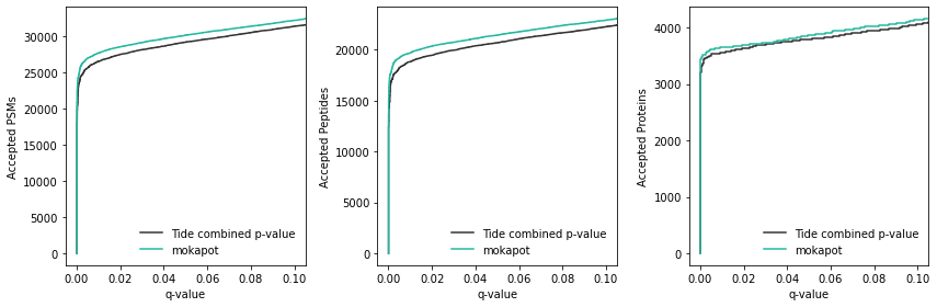
Excellent. It looks like mokapot increased our power to detect a few hundred more PSMs and peptides at 1% FDR. We figure out the exact improvement by looking at the data:

# PSMs
moka_psms = (moka_conf.psms["mokapot q-value"] <= 0.01).sum()
tide_psms = (tide_conf.psms["mokapot q-value"] <= 0.01).sum()
print(f"PSMs gained by mokapot: {moka_psms - tide_psms}")

# Peptides
moka_peps = (moka_conf.peptides["mokapot q-value"] <= 0.01).sum()
tide_peps = (tide_conf.peptides["mokapot q-value"] <= 0.01).sum()
print(f"Peptides gained by mokapot: {moka_peps - tide_peps}")

# Proteins
moka_prots = (moka_conf.proteins["mokapot q-value"] <= 0.01).sum()
tide_prots = (tide_conf.proteins["mokapot q-value"] <= 0.01).sum()
print(f"Proteins gained by mokapot: {moka_prots - tide_prots}")

PSMs gained by mokapot: 1149
Peptides gained by mokapot: 872
Proteins gained by mokapot: 89

Finally, we will save the results as tab-delimited text files:

result_files = moka_conf.to_txt(dest_dir=out_dir)
result_files

['basic_python_api_output/mokapot.psms.txt',
 'basic_python_api_output/mokapot.peptides.txt',
 'basic_python_api_output/mokapot.proteins.txt']

Wrapping up

This vignette demonstrated the basic usage of mokapot’s Python API. For more detail about any of the mokapot functions and classes that we used, see the mokapot Python API documentation. Finally, check out the other vignettes for examples of advanced usage of mokapot’s Python API.